Statistical analysis

Find the signal.
Make it useful.

Explore variation, understand relationships and turn an analytical result into something the whole engineering team can see.

See the shape of the data

Start with
a better question.

Move from the distribution to grouped variation and probability views. Keep the summary close to the picture.

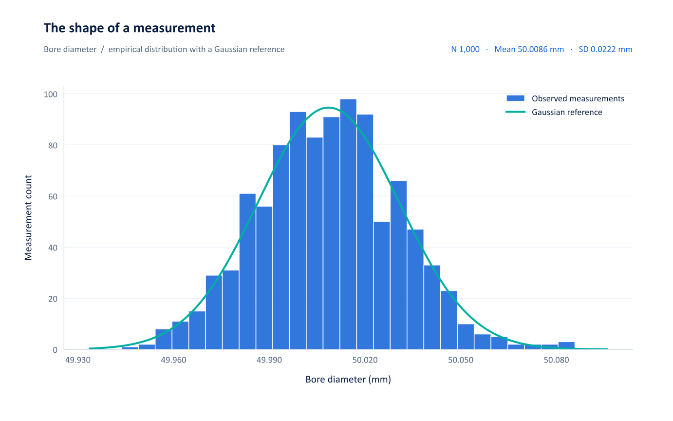
Measurement distributionNUMETIVA
Histogram of 1,000 bore-diameter measurements with a Gaussian reference and numerical summary.

Relationships & predictive models

Follow the response.
Explore what changes.

Connect scatter plots and fitted models with interactive profilers. Explore how predictor settings relate to the modelled response, then retain the useful view in your project.

  • Regression and response exploration
  • Tree, forest and neural-network workflows
  • Related diagnostics and model output
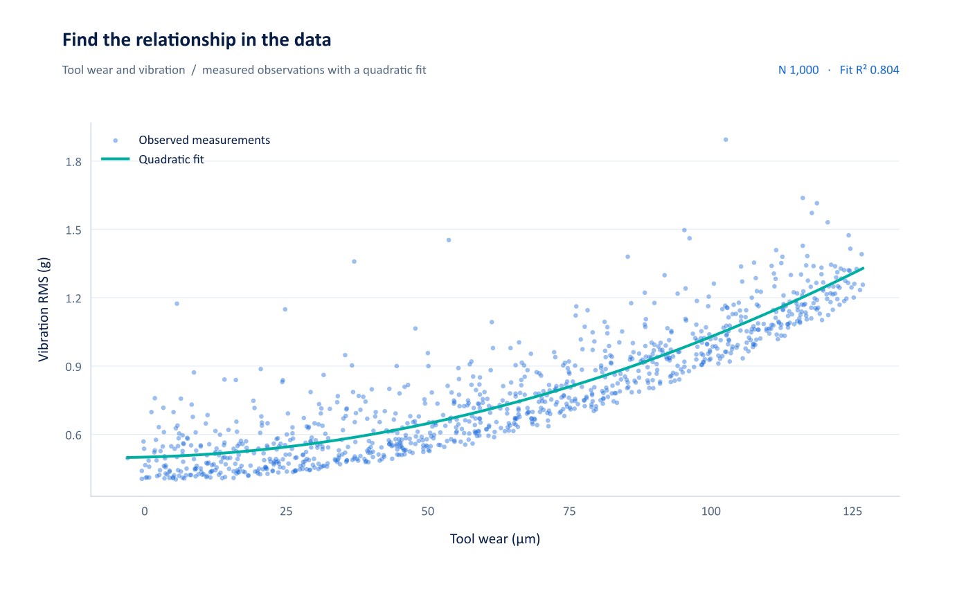
Wear & vibrationNUMETIVA
Python-generated scatter plot showing the relationship between tool wear and vibration in the engineering demonstration dataset.

Predictive exploration / application scene views

The response.
Right beside the predictors.

Move between a neural network, a random forest and regression diagnostics. Inspect the shape of the fitted response and what the residuals reveal.

Neural network profilerNUMETIVA
Numetiva saved-scene vector view: neural network prediction profiler showing the response Y against X, Z and Line, with the selected predictor settings marked.
01 / RESPONSE

See what changes.

Profiler panels place the modelled response against each predictor.

02 / SETTINGS

Keep the context.

Reference lines show the selected settings in each saved view.

03 / REVIEW

Ask the next question.

Return to the model output and diagnostics before taking a result forward.

The language of quality

Location. Spread.
Stability. Capability.

Bring descriptive statistics, control charts and capability views into the same engineering conversation.

01

Understand the measurement.

Distributions, box plots and grouped comparisons make the variation visible.

02

Follow the process.

Use control and time-ordered views to inspect behaviour across the recorded sequence.

03

Share the useful result.

Export clear charts and supporting text to Word, PowerPoint and PDF.

Capability / application scene view

One result.
Several essential perspectives.

Location, spread, stability and nonconformance in a connected diagnostic view. Keep within-process and overall estimates visible together.

Capability diagnostic dashboardNUMETIVA
Numetiva saved-scene vector view: capability diagnostic dashboard showing process location, moving range, distribution, normal probability, capability indices and observed versus modelled PPM.

Bring your engineering question.

Explore how Numetiva fits your data, workflow and review requirements.

Talk to Numetiva
Numetiva / vector chart
100%Open SVG ↗

Zoom for individual dies and labels. Drag or scroll to pan. + / - to zoom; 0 to fit.

Numetiva / interactive product tour

From a question to a checked output

Your question.
A reviewable script.

Use the assistant to draft Python, inspect the code in the workbench, then run it against your worksheet. Bring the latest error into Review / fix when the script needs attention.

  1. 01
    Ask with context.

    Name the response, predictors and the chart you need.

  2. 02
    Inspect the draft.

    Check the column names, transformations and method.

  3. 03
    Run and review.

    Use the returned output and errors to guide the next step.

Explore AI & Python
Python / exampleWorksheet context
import numpy as np
import matplotlib.pyplot as plt

x = df["Tool_Wear_um"].to_numpy()
y = df["Vibration_RMS_g"].to_numpy()
valid = np.isfinite(x) & np.isfinite(y)
x, y = x[valid], y[valid]

fig, ax = plt.subplots()
ax.scatter(x, y, s=18, alpha=0.7)
coefficients = np.polyfit(x, y, 2)
grid = np.linspace(x.min(), x.max(), 200)
ax.plot(grid, np.polyval(coefficients, grid))
ax.set(xlabel="Tool wear / µm",
       ylabel="Vibration / g")
plt.show()
About this product tour